Thoughts: ESRI Developer Summit 2014

Last week I attended the ESRI Developer Summit in Palm Springs, CA.  This was my first venture inside the ESRI world, and I came away impressed.  As a in my office, it’s not always easy to stay ahead of the technology curve.  After 4 days at the conference I feel that not only am I up to date on all things ESRI, but that I can also see clearly where they are headed in the near future.

Trends:

ArcGIS Online:  In one of the JavaScript sessions, a presenter asked for a show of hands on who was using ArcGIS Online.  It looked like somewhere between half to three-forths of the attendees had their hand up.  Of course, I don’t mean this to be a reflection of the GIS world as a whole, but rather to give some perspective; it might not be a stretch to think that ESRI already has quite a few more AGOL subscriptions than ArcGIS Server accounts.  So it is not just with a sense of optimism that ESRI seems to be orienting their future plans around AGOL, the JavaScript API and web mapping.

Javascript: In February ESRI released their roadmap whereby they announced they would be discontinuing further development with Silverlight and Flex in favor of their JavaScript API.  It appeared that people were starting to catch on.  There were a couple of sessions introducing the JavaScript API in addition to classes instructing users how to transition out of Flex and into JavaScript.

Lest you think ESRI was solely courting the JavaScript noob, there were also a multitude of advanced sessions.  The demonstration of using Angular (a JavaScript framework created by Google) was cool enough that even though it was well over my head, I keep returning to it to see if I can figure out how to bend it to my will.

As far as JS API improvements, the most useful to me is the canvas blending functionality.  (Sorry, no link)  For those exclusively using the JS API (rather than out-of-the-box ArcGIS Online or ArcGIS Server, which will allow you to create ‘map sandwiches‘), we have had to endure the rather clunky design of having our translucent polygon features obscure the labeling of the standard basemaps.  With canvas blending (predicted for version 4.0 of the API), the basemap labels showed through the features clearly.

Additionally, the JS API debuted many cool new symbolization capabilities including a continuous color scale, a dot-density renderer, and label layers.  You can view more about the JavaScript API here and here.

Github:  It was telling that the very first session on the very first day of the conference was ‘Intro to Github’.  Perhaps that’s to be expected when your keynote speaker is Chris Wanstrath, who founded the company.  However, as it turned out, ESRI was not just throwing a bone to their keynoter – they really are obsessed.  ESRI has truly embraced Github. Perhaps if you’re picky with semantics they haven’t embraced open-source (per the naysayers), but they certainly have taken to social coding.

The vast majority of the sessions provided links to Github repositories where examples and utilities were stored.  It was clear that the code was not posted as an afterthought (or under orders), presenters genuinely encouraged participation.

While I have noticed ESRI’s Github repositories for some time now, I had no idea of the breadth of projects that were out there.  ESRI-Leaflet and ESRI-Bootstrap will almost certainly find their way into my upcoming webmaps.


Previews:

The new Webmap Builder was a big hit.  If you’ve spent any time working with ArcGIS Online, you’re probably aware that AGOL can create some pretty clunky looking webmaps.  Additionally, the creative options are rather limited.  The out-of-the-box functionality creates maps that mostly fall into the category of: “here is my data, click for a popup”.  Anything beyond that will require some programming chops. This is where the Webmap Builder shines.  It creates a more highly customized application that does not require any coding whatsoever (though you are free to embellish the apps with your own code if you choose).  As you can imagine, there are a lot of people who do not have the time or energy to work their way up the steep learning curve of coding, and this will be a game changer for them.  However, seasoned programmers have no reason to fret.  As one ESRI speaker put it, “We’ve made it very easy to create web maps.  But don’t worry, not too easy.  You’ll still have a job.”  Thanks.

ArcGIS Professional: This is the new desktop client – or – if you listen to ESRI, an additional desktop client option that you will receive in addition to ArcGIS Desktop.  In my opinion this will replace ArcGIS Desktop altogether within 2-3 years.  The integration with ArcGIS Online is a lot tighter. One (or two) click publishing to the web will be a reality.  The AGOL workflow as it is now is a bit clunky, with the uploading of shapefiles, and the re-uploading of shapefiles again when your boss wants to add another attribute.  ArcGIS Pro will significantly improve that experience, all while preserving the core functionality that most Desktop users are familiar with.

3D: I rarely work in 3D, so the first few times they mentioned it in the plenary I tuned out. I didn’t see a use case for it, and ESRI’s previous 3D offerings seemed fairly lackluster to me. But after seeing multiple demo’s, and even integration into the JS API, I can see a lot of data visualization type projects where it could be useful. 3D web-app animations, for one, would be an awesome way to visualize some of the demographic trends that I work on. ArcGIS Pro even appeared to have a full suite of 3D features.  And all of the examples I saw, (both on Pro and the JS API) looked surprisingly zippy.

Other Notes:

Dojo is still decidedly unpopular. So why Dojo? The question was asked in a session, and rather than try to reconstruct the verbatim response, I think the long and short of it is that this was a decision made back in 2007, and now the JavaScript API and Dojo are inextricably intertwined.  It is a bit troubling to me that instead of trying to extract themselves from Dojo, they seem to be doubling-down.

A colleague pointed out that ESRI may be the only thing keeping Dojo from slipping into oblivion.  Seems likely.


 In Closing…

All things considered, it was a very fun and informative conference.  It’s really quite the of coding and mapping enthusiasts.  Where else can you find people who drop ‘feature class’ and ‘api’ in casual conversation?  Those are my type of folk.  With any luck I’ll be back next year!

Posted in Uncategorized | Leave a comment

Census Reporter Amazon EC2 with TileMill and MapBox

My latest blog posts have been purely about accessing Census Reporter data.  That’s important as a foundation, but now it’s time to bring it all together and see how we can use this resource (and other amazing resources out there such as TileMill and MapBox) to create useful and informative projects.

In this post we’ll take advantage of TileMill and MapBox to create a map of Median Home Value for US Metropolitan Areas (the CBSA Census Geography ).

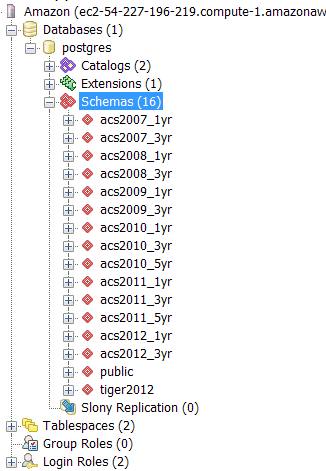
First, follow steps 1-5 here to boot up an instance of the Census Reporter Database.

Next, follow the post here to connect to PgAdmin.

Download and Install Tilemill.

Create a free MapBox account.  (The Sign Up button is in the upper right corner).


Let’s start by creating the geographic data layer that we will use in TileMill.  We will be doing this in PgAdmin using the SQL Query tool.

Let’s start by joining the data fields to the census geographic header file.

CREATE TABLE public.CBSA_Pop AS
SELECT tiger2012.cbsa.gid, tiger2012.cbsa.namelsad, tiger2012.cbsa.cbsafp, tiger2012.cbsa.the_geom, acs2012_3yr.geoheader.geoid, acs2012_3yr.geoheader.sumlevel FROM acs2012_3yr.geoheader, tiger2012.cbsa WHERE acs2012_3yr.geoheader.cbsa = tiger2012.cbsa.cbsafp and acs2012_3yr.geoheader.sumlevel=310;

Next we’ll assign the gid field to be the primary key.

ALTER TABLE public.CBSA_Pop ADD PRIMARY KEY (gid);

Now that we have our data, we’ll want to join it to the geography layer.

CREATE TABLE public.CBSA_TileMill2 AS
SELECT public.CBSA_Pop.gid, public.CBSA_Pop.namelsad, public.CBSA_Pop.cbsafp, public.CBSA_Pop.the_geom, public.CBSA_Pop.geoid, acs2012_3yr.seq0155.b25077001 FROM public.CBSA_Pop, acs2012_3yr.seq0155
WHERE public.CBSA_Pop.geoid = acs2012_3yr.seq0155.geoid;

Again, we’ll assign gid to be the primary key

ALTER TABLE public.CBSA_TileMill2 ADD PRIMARY KEY (gid);

Then we’ll add a spatial index to the new layer.

CREATE INDEX geomindex ON public.cbsa_tilemill2 USING GIST ( the_geom );

Data creation finished!  Anyone who is familiar with working with Census Data knows that the above step could have taken upwards of 30 minutes normally (if we were using a typical workflow whereby we were downloading through American Fact Finder and joining to our TIGER layers in ArcMap before uploading to our database.)  And not that the above SQL was terribly burdensome, but an individual much more skilled in SQL than I am could have done it even more concisely.

Next up; let’s load our data into TileMill and style it.

Open TileMill, and start a new project.

Fill out the project details so that they look something like this:

Now, open your project.  You should be looking at an essentially empty map of the world.  Let’s add some data!  Find the Layers button in the lower left corner.  It looks like this:

Click ‘Add Layer’, click on the ‘PostGIS’ button at the top right, and then fill out the dialog as follows:

Your connection string should read:

host=ec2-54-224-74-22.compute-1.amazonaws.com port=5432 user=census password=censuspassword dbname=census

(Of course – don’t copy exactly, substitute your own Amazon Public DNS)

Enter the other values as you’ve seen them above.  Don’t worry about copying the SRS string exactly.  Just choose WGS84 and everything will populate automagically.

Press Save to return to the map.  You can’t see anything because we haven’t styled this layer yet.

Let’s add some CartoCSS to style this layer based upon the Median Home Value (field: b25077001) for each Metro.

#cbsa {
 line-color:#594;
 line-width:0.5;
 polygon-opacity:1;
 polygon-fill:#99FFFF;
 [b25077001 >= 50000] { polygon-fill:#99DDFF; }
 [b25077001 >= 75000] { polygon-fill:#99BBFF; }
 [b25077001 >= 100000] { polygon-fill:#9999FF; }
 [b25077001 >= 125000] { polygon-fill:#9977FF; }
 [b25077001 >= 150000] { polygon-fill:#9955FF; }
 [b25077001 >= 175000] { polygon-fill:#9933FF; }
 [b25077001 >= 200000] { polygon-fill:#9911FF; }
 [b25077001 >= 225000] { polygon-fill:#9900EE; }
 [b25077001 >= 250000] { polygon-fill:#9900CC; }
 [b25077001 >= 275000] { polygon-fill:#9900AA; }
 [b25077001 >= 300000] { polygon-fill:#990088; }
 [b25077001 >= 325000] { polygon-fill:#990066; }
 [b25077001 >= 350000] { polygon-fill:#990044; }
 [b25077001 >= 375000] { polygon-fill:#990022; }
 [b25077001 >= 400000] { polygon-fill:#990000; }
 }

Press the save button in the top right corner.  Be patient… TileMill is gathering a lot of data from your cloud database right now.  After a short while, the map should be fully loaded:

Fantastic.  You can use what you’ve learned to go nuts and add a State Layer if you want. (tiger2012.state)  Symbolize it with a black outline (or whatever).  I’ll skip this step for brevity.

(You may want to consider uploading the Census cartographic boundary files. Otherwise Michigan looks even more awkward than it already is).

Let’s add a couple more TileMill features.

First up: adding mouseover ability

Click the Templates button.  Make sure the ‘Teaser’ tab is selected.  Next, look near the bottom of the screen and choose the layer ‘cbsa’.

In the text area, type:

{{{namelsad}}} <br />
Median Value: {{{b25077001}}}

Press Save (in the upper right corner of the TileMill application).

Next, to add the legend.

Click the legend tab, if you haven’t already.  I’ve created some code for the legend to save you some time (based off of a MapBox sample that’s been modified).

<div class='my-legend'>
<div class='legend-title'>Median Value (Owner Occupied Housing Units)</div>
<div class='legend-scale'>
 <ul class='legend-labels'>
 <li><span style='background:#99FFFF;'></span><$50k</li>
 <li><span style='background:#99DDFF;'></span></li>
 <li><span style='background:#99BBFF;'></span></li>
 <li><span style='background:#9999FF;'></span></li>
 <li><span style='background:#9977FF;'></span></li>
 <li><span style='background:#9955FF;'></span></li>
 <li><span style='background:#9933FF;'></span></li>
 <li><span style='background:#9911FF;'></span></li>
 <li><span style='background:#9900EE;'></span></li>
 <li><span style='background:#9900CC;'></span></li>
 <li><span style='background:#9900AA;'></span></li>
 <li><span style='background:#990088;'></span></li>
 <li><span style='background:#990066;'></span></li>
 <li><span style='background:#990044;'></span></li>
 <li><span style='background:#990022;'></span>>$400k</li>
 <li><span style='background:#990000;'></span></li>
 </ul>
</div>
<div class='legend-source'>Source: <a href="http://www.census.gov/acs/www/">American Community Survey 2012 3-Year Estimates</a></div>
</div>
<style type='text/css'>
 .my-legend .legend-title {
 text-align: left;
 margin-bottom: 8px;
 font-weight: bold;
 font-size: 90%;
 }
 .my-legend .legend-scale ul {
 margin: 0;
 padding: 0;
 float: left;
 list-style: none;
 }
 .my-legend .legend-scale ul li {
 display: block;
 float: left;
 width: 15px;
 margin-bottom: 6px;
 text-align: center;
 font-size: 80%;
 list-style: none;
 }
 .my-legend ul.legend-labels li span {
 display: block;
 float: left;
 height: 15px;
 width: 15px;
 }
 .my-legend .legend-source {
 font-size: 70%;
 color: #999;
 clear: both;
 }
 .my-legend a {
 color: #777;
 }
</style>

Press Save in the upper right corner of TileMill, then exit the Templates screen.

With those easy steps, we’ve now added some much needed extra functionality to our map.  The legend is clearly visible in the lower right corner.  Also, if you mouse-over a metro area, you’ll see that median home values are shown in a box on the top right corner of the map window.

So uh, we have an extremely slow to load map that is currently confined to our personal computer.  Let’s change that.

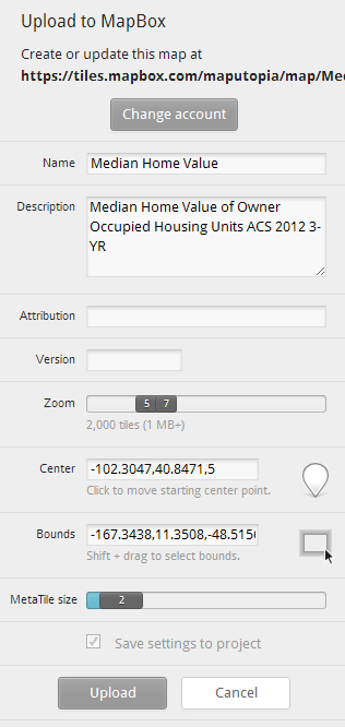
Click the Export button in the upper-right corner of your TileMill application.  On the drop down menu, select Upload.

Play around with the extent and the Zoom Levels. (especially the zoom levels)  The free version of the MapBox account does have some limits, so you’ll want to keep the size of this project small.

Wait until everything is finished uploading.  Then go ahead and press the View button.

Voila!

Posted in Uncategorized | Leave a comment

Connect Amazon EC2 to PgAdmin

In my previous post I gave some detailed instructions on how to connect Census Reporter’s EC2 database to MS Access.  While sufficient for the purposes of most demographers, I realize that some may prefer to access the database in a much more direct way.  You can easily connect directly to PgAdmin III if you prefer, here’s what you need to do:

Refer to my previous blog post and make sure to follow steps 4 and 5.  PgAdmin will not be able to see your database if the security settings aren’t adjusted, so don’t skip these steps!

When adding a new connection, here’s what your PgAdmin III connection dialog should look like.

The password is ‘censuspassword’.

*To find the name of your Host, look back on your instance page and copy the Public DNS.

With any luck, you should be looking at this:


Posted in Uncategorized | Leave a comment

Using Census Reporter’s Amazon EC2 Database

Welcome to your new American Community Survey Data platform.

For most demographers, ‘the cloud’ and ‘big data’ are nothing more than corporate buzzwords, often found in various combinations with business-speak nonsense such as ‘best practices’ and ‘leveraging core competencies’.  Most of the time we’re consumed with our comfortable world of American Fact Finder searches and Microsoft Access queries, and that suits our purposes just fine.  We’re all isolated in our various niche’s – but since we all essentially rely on the same data to do our jobs, there ends up being an excessive duplication of effort.  Of course, it doesn’t have to be that way.

The brilliant folks at www.censusreporter.org, a census data resource for journalists, have finally succeeded in making American Community Survey data available to the masses (that’s us).  They have compiled an extensive database spanning the years 2005-2012, including the most current 1-year, 3-year, and 5-year datasets.   for a diagram of the data currently available.

Imagine being able to instantly pull data tables from the latest 5-year release without having to spend hours downloading and formatting an unwieldy chunk of data.  That work has already been done – you may as well take advantage of it.  The only thing you have to do is follow a few easy instructions to set up your server in the cloud.

Did I say easy?  Kinda easy.  Relatively easy.  Okay, perhaps a little intimidating to those not familiar with the technology.  But that’s why I’m here; to walk you through each step of the process.  These are instructions adapted from Census Reporter’s blog post , that I have updated to reflect changes to Amazon’s interface.  I’ve also added additional instructions so that demographers will be able to use the data with the tool they are most comfortable with; namely, Microsoft Access.

Step 1.  .  This is the only step I’m not going to hold your hand through.  Just click the orange ‘Sign Up’ button at the top-center of the page.  You’re going to end up spending some money, so you’ll probably need to put in some credit card information at some point.  The good news is that you can test this whole setup for a few days and probably spend less than $5.  Or you can just try this tutorial, decide it’s not for you, and likely spend less than $1.

Step 2.  Now that you’ve created an account, you’re going to want to visit your .  There’s a lot of crazy stuff on that page, but don’t worry. The only item that interests you is EC2.  Click on it.
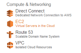
This will take you to the EC2 dashboard page.  There’s no sense explaining too much of this right now.  Let’s just dive in.  Click ‘Launch Instance’ to start.

You’ve now been taken to a page where you’ll be asked to choose which Amazon Machine Image (AMI) you would like to use.

Before you do anything else, please refer to the upper-right corner of your webpage and choose N.Virginia for the geographic region.  (TMI: For whatever reason, when I created this tutorial the snapshot of the census reporter database wasn’t available in some of the other regions.)

Now, back to picking out our AMI.  This is somewhat like choosing what type of computer you want to run your database on in the cloud.  Census Reporter recommends you choose the Ubuntu Server 12.04.3 LTS.

Make sure 64-bit is selected, and then press the ‘Select’ button.

On the next page, you’ll be asked to choose an Instance Type.  This is like asking how powerful you want your computer to be.  I would suggest choosing one of the General Purpose instances.  Choose at least the General Purpose m1.medium instance.  Don’t be lured by the ‘Free Tier’ instances in hopes that you can get through this without spending just a tiny amount of money.  (You can’t.)

Here’s what my selection looked like:
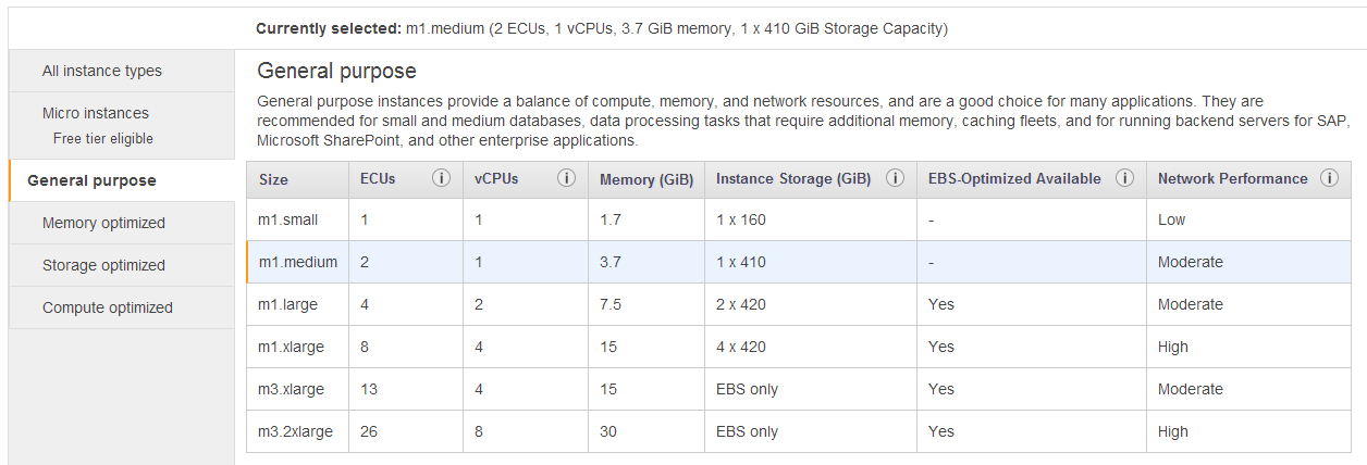
Now click ‘Configure Instance Details’ in the lower right corner to move on to the next screen.

 Leave everything default on the Configure Instance Details Page.  Then click the ‘Next: Add Storage’ button.
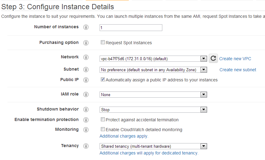
Now you should be on the ‘Add Storage’ page.  This one is important, so make sure you get all the details correct.  Think of this section as adding your database.  You’re going to be adding a copy (snapshot) of Census Reporter’s database.

Choose EBS for Type.  Choose /dev/sdc for Device.  Type: snap-f17240e0 into Snapshot.  Type 500 into Size (GB), and click on the box that says ‘Delete on Termination’.

Then click the button on the lower right that says ‘Next: Tag Instance’.

Keep everything default on this page, then go to next page: ‘Next: Configure Security Group’.

We’ll revisit the Security Group settings in a few more minutes.  For now, leave everything default.  Let’s get this show on the road.  Click ‘Review and Launch’ here, and then on the next page, click ‘Launch’.

Next up you’ll get a dialog box about Key Pairs.  You will need this file to be able to log in to your instance.  Choose ‘Create New Key Pair’ in the first drop-down list.  Name your Key Pair something hopefully not as obscure as ‘AWS_KP’ and click the ‘Download Key Pair’ button.  You should probably get some sort of Save File notification.  Put this file somewhere that you will remember!  This is important!
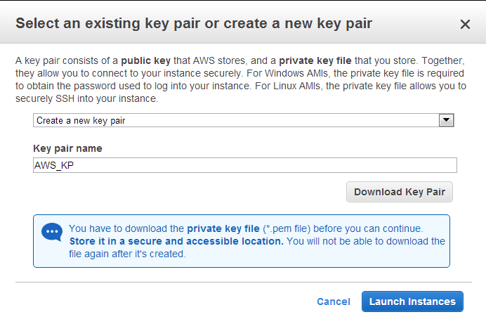
Lastly, press the ‘Launch Instances’ button.

The next page will let you know that Amazon is setting up your Instance.  Click the blue ‘View Instances’ button in the lower corner of the page.

Keep an eye on this screen.  Once the ‘Status Checks’ field reads ‘2/2 checks passed’, then you’re ready for Step 3.  (This will take a few minutes).

Step 3.  Now that your instance has been created by Amazon, you’re going to be typing a few commands so that everything will be connected behind the scenes.  Check the box next to your instance, and press the ‘Connect’ button. 
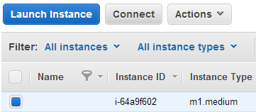
The next dialog box will ask you how you plan to connect.  Change the selected option to: ‘A Java SSH Client directly from my browser’.
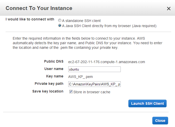
Find the key on your hard drive.  Type in the exact path: (in my case) ‘C:AmazonKeyPairsAWS_KP_.pem’.  Then press ‘Launch SSH Client’.

A small dialog box will pop up the first time that you connect this way, asking if you want to add this host to your set of known hosts.  Click ‘Yes’.

(We can ‘Close’ our ‘Connect your Instance’ dialog box now.  We won’t need it anymore.)

Even if you’re fairly techy, this may be the part where you feel as if you’re falling down the rabbit hole.  Just hang in there.  I’ll try to let you know what’s going on in plain English.  (And where I have no clue, I’ll just give you the next instruction).

The dreaded command line dialog opens up.  So where are we?  Right now, we’re talking directly to our cloud computer, which is a Linux machine. (Thus we’ll have to speak in a language quite different than what we’re used to).

This is the first command we (very carefully) type in:

curl -fsSL https://raw.github.com/censusreporter/census-postgres-scripts/master/00_connect_ebs_volume.sh | tail -n 3 | sed 's/xvdf/xvdc/g' | sh

When that is finished, enter this (all on one line):

curl -fsSL https://raw.github.com/censusreporter/census-postgres- 
scripts/c1a8cefb6e1afda7f5f706c15b7fef43d114b242/01_set_up_postgresql.sh | tail -n 9 | sudo sh

This will process for a while.  (Note: this script is different from the one suggested at the Census Reporter site.  For whatever reason, the script from their instructions no longer works.  The one here – which does work as of 1/18/14 – is essentially a link to a previous version of their script.  I’ll update this post as needed as versions change. )

Be patient and wait until you’re greeted with a ‘~$’ prompt. When that happens, we will attempt to log into the database.  Type in:

psql -U census -h localhost postgres

When prompted for your password, type in: censuspassword
(Note that your keypresses are being recorded, even though nothing is shown).

So what just happened?  The database (a PostgreSQL database) was installed and configured.  In the last line you typed, you actually logged into the database.  (You’ll know that you’re successfully logged in if the command prompt changed to ‘postgres=> ‘ ).

If you were a super advanced user, you could stop there.  For the rest of us who prefer not to work at the command line, you will need to change some security settings so that you can interact with the database in a more familiar environment.  The catch is that you’ll be altering the security settings of the cloud computer in a Linux environment.

We’re not actually going to be working in PostgreSQL for now, so we can type the following command to exit the database and return to the Linux command prompt:

q

Step 4.  We’ll need to change some security group settings.  Go back to the ‘Instances’ web page, check the box next to your Instance, and look down at the tabbed area below.
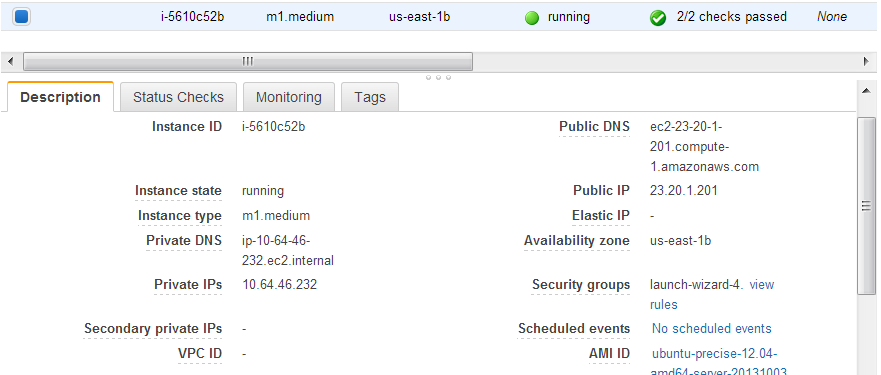
Take a look where it says ‘Security Groups’ on the right hand side.  Mine says ‘launch-wizard-4′.  Yours will say something different (most likely).  Take note of this name.

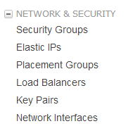
Next, on the left side of the page, locate where it says ‘Security Groups’ (under the NETWORK & SECURITY section).  Click there.
On the Security Group page, click on the Security Group Name we noted previously.  Then, on the bottom click on the Inbound tab.  Type 5432 into the Port Range.  Then for the Source, enter in your IP address, followed by /32.  (essentially, replace the x.x.x.x with your IP address.  If you don’t know what your IP address is, you can literally google ‘What is my IP address?’ and Google will tell you.)
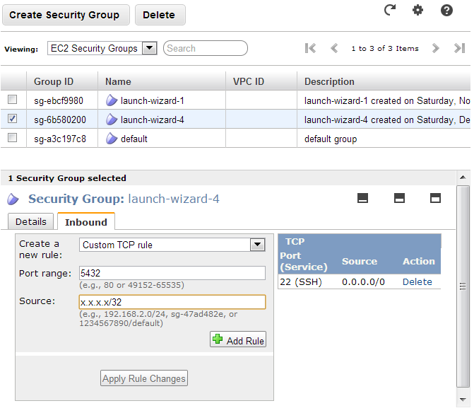
Don’t forget to press the Add Rule button, then the Apply Rule Changes button.

Step 5.  This is the hardest step.  You’re going to need to alter some files on the server. Let’s return to the command line.  (You may need to Connect again on the Instances page as you did previously).

 You first need to navigate to the directory with the configuration files.  Type in:

cd /etc/postgresql/9.1/main

then type in:

ls

The command ls will list the files in your current directory.  If all went well, you should see the following:

 Next up, we’re going to be editing the pg_hba.conf file using a program called Vim.  The command to edit this file with Vim is:

sudo vi pg_hba.conf

This will open up the file for editing.  Now press the ‘i’ key on your keyboard.  This toggles Insert mode, and will allow you to make edits.

Scroll down (with the arrow keys) and edit the file so that it looks like the following:
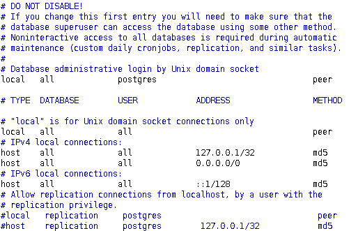
Essentially, what you’re doing is finding the line that reads:

host        all         all      127.0.0.1/32        md5

And adding the following line below it:

host        all         all      0.0.0.0/0        md5

Now to save and quit, Press ESCAPE, then type:

:wq

This should take you back to the familiar command prompt.

We still have one more file to edit, postgresql.conf.  Type:

sudo vi postgresql.conf

Scroll down to the line that looks like this:

And edit it (remember to press the ‘i’ key to enter Insert mode) to look like this:


Now to save and quit, Press ESCAPE, then type:

:wq

Breath a sigh of relief, you’re almost done.  The last step is to restart PostgreSQL to incorporate these changes.  Type:

sudo /etc/init.d/postgresql restart

Then you’re done with the command line.  Lastly, type:

exit

And close the window.


Step 6.  Let’s connect to Microsoft Access!

Not so fast!  You need to install a driver first.  Go to this page to download the PostgreSQL ODBC driver that will allow you to connect a PostgreSQL database to Microsoft Access.  My version of MS Access is 32-bit, so I chose the 32-bit version of the latest driver psqlodbc_09_02_0100.zip . (In retrospect, perhaps I should have chosen the 9.1 version of the driver, since that is the version of PostgreSQL on the Linux machine.  No matter, there seems to be some backwards compatibility because it works fine.)

Download and install that driver.  Your mileage may vary slightly from these directions if you have a 64 bit version of MS Access.

Step 7.  NOW Let’s connect to Microsoft Access!

Open MS Access and create a New Blank Database.  Depending on your version of MS Access, these instructions may vary slightly.  For me (using the Ribbon in Access 2010), I click on the ‘External Data’ section and then click on the ‘ODBC Database’ Icon.
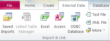
 

Then you’ll select ‘Link to the data source by creating a linked table’. (You can choose to Import the data instead – your database will just fill up faster because you will actually be downloading the data from Amazon, rather than just referencing it).


Then you’ll click the Machine Data Source tab, and press the ‘New…’ button.

You can choose whichever option that you want for this dialog, depending on your User Account preferences.  Press Next.

On the ‘Create New Data Source’ dialog, scroll down and select PostgreSQL ANSI, and then press Next.
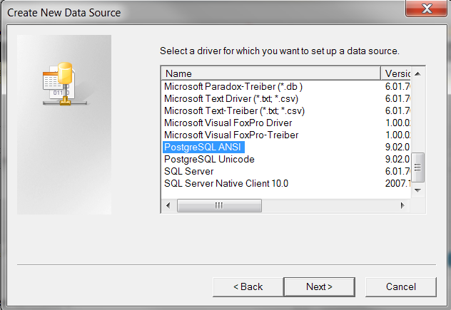
Click ‘Finish’.  Here’s the next dialog:
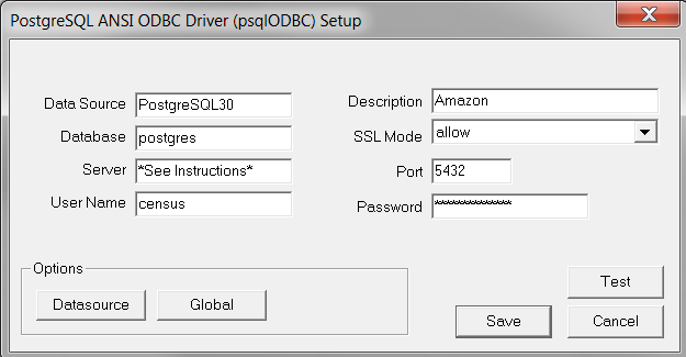
 

Fill out the dialog box exactly how it shows in the picture above, with two important notes;

1.  The password is censuspassword.

2.  For the Server information, you’ll need to return to your EC2 instance webpage, click your instance, and look in the top right of the information panel for your Public DNS information.

3. Click the Datasource button and Uncheck ‘Use Declare/Fetch’.  Press Apply then OK.

Press Test.  Hopefully you’ll get a popup dialog that says ‘Connection successful’.

Press Okay, then press Save.

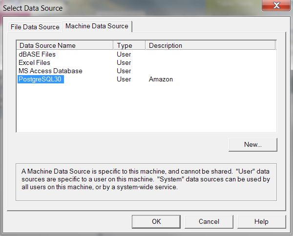
Now, back at the ‘Select Data Source’ dialog, highlight ‘PostgreSQL30′ and press ‘OK’.
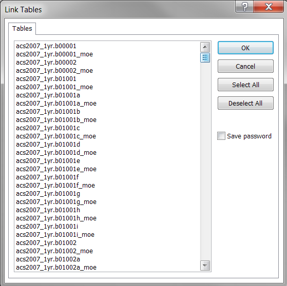
Voila!  Hundreds of ACS Tables!  You can probably take it from here.  Don’t forget, if you’re curious about which data tables are in which files, you can look that up easily in the documentation files on the Census FTP site.
 

Final Notes:  To avoid being charged extra, make sure to terminate your instance when you’re done with it.  You can choose to stop your instance instead (so that you won’t have to run through this process again), but stopping an instance – while saving some money – will not stop you from being charged entirely.  Amazon will still be charging you for database storage (the EBS volume).

Stopping and starting your instance will very likely change your public DNS.  Thus be prepared to change your MS Access PostgreSQL login information each time you do this.

Advanced Users:  Instructions on connecting to pgAdmin and on using PHP to connect to the database are forthcoming.  Much of the setup instructions (minus the MS Access pieces) are the same.

Posted in Uncategorized | Leave a comment

Bruce Springsteen – Touring Heat Map

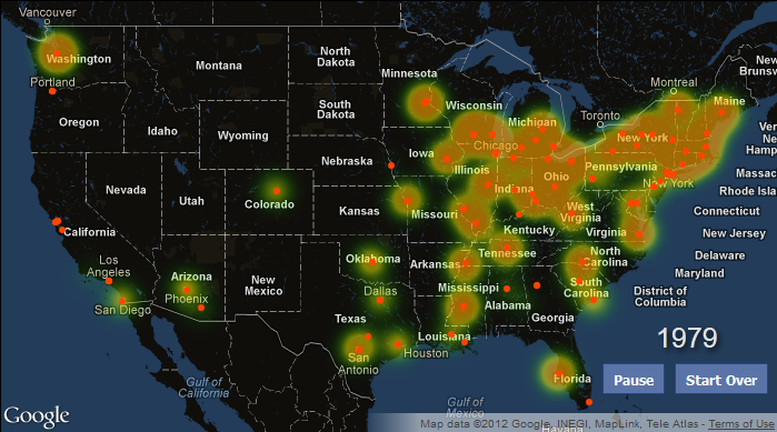
Heat Map

Springsteen Touring Heat Map - Click for Animation

My latest project has been to take a career’s worth of Bruce Springsteen tour dates (data courtesy of The Timoney Group) and try to make sense of it all.  While I admit to being just a casual fan of Springsteen, working on this project has given me an understanding of the tireless performer he is.  The data encompasses more than 1,500 tour dates over 40 years.  In the beginning of his career, in fact, he would often perform multiple shows in one night.

Behind the scenes, the main map is a just a stylized version of the familiar google map interface that we all know and love.  Data is loaded from two JSON files; concert dates and album information.  The construction of the Heat Map itself is handled by feeding the data to a Google HeatMap layer (part of the ).  The tricky part is the animation.  While constructing a static Heat Map is a piece of cake, Google does not provide any quick and easy built-in functions or methods to accommodate animation.  Luckily, Google does provide something called an MVC Array. By using this type of array as the data source for the Heat Map, we can add and remove concert data and have these changes dynamically reflected in the HeatMap layer.

Aside from that complex piece of javascript, it’s mostly just a matter of some simple html and css to construct the layout.  The scrolling ticker of venues is a jquery plugin.

The intensity of the heat map is based on relative popularity.  Since the East Coast is very densely populated, any band would seem wildly popular there compared to the rest of the country.  The solution is to weight the size of the concert relative to the surrounding metropolitan area.  Thus, the heat map intensity of an arena show in New York City (pop. ~9,000,000) is just a flash in the pan compared to that of any show in Iowa City (pop. ~150,000).  Still, even with this adjustment Springsteen’s popularity in the Northeast and in the Rust Belt can’t be overstated.

Click here to view the animation.  A great writeup based on this visualization can be found here.

And, if you’re curious, Springsteen is on tour right now.

Posted in Uncategorized | 2 Comments